6. Camera Hardware
This chapter provides an overview of how the camera works under various conditions, as well as an introduction to the software interface that picamera uses.
6.1. Theory of Operation
Many questions I receive regarding picamera are based on misunderstandings of how the camera works. This chapter attempts to correct those misunderstandings and gives the reader a basic description of the operation of the camera. The chapter deliberately follows a lie-to-children model, presenting first a technically inaccurate but useful model of the camera’s operation, then refining it closer to the truth later on.
6.1.1. Misconception #1
The Pi’s camera module is basically a mobile phone camera module. Mobile phone digital cameras differ from larger, more expensive, cameras (DSLRs) in a few respects. The most important of these, for understanding the Pi’s camera, is that many mobile cameras (including the Pi’s camera module) use a rolling shutter to capture images. When the camera needs to capture an image, it reads out pixels from the sensor a row at a time rather than capturing all pixel values at once.
In fact, the “global shutter” on DSLRs typically also reads out pixels a row at a time. The major difference is that a DSLR will have a physical shutter that covers the sensor. Hence in a DSLR the procedure for capturing an image is to open the shutter, letting the sensor “view” the scene, close the shutter, then read out each line from the sensor.
The notion of “capturing an image” is thus a bit misleading as what we actually mean is “reading each row from the sensor in turn and assembling them back into an image”.
6.1.2. Misconception #2
The notion that the camera is effectively idle until we tell it to capture a frame is also misleading. Don’t think of the camera as a still image camera. Think of it as a video camera. Specifically one that, as soon as it is initialized, is constantly streaming frames (or rather rows of frames) down the ribbon cable to the Pi for processing.
The camera may seem idle, and your script may be doing nothing with the camera, but still numerous tasks are going on in the background (automatic gain control, exposure time, white balance, and several other tasks which we’ll cover later on).
This background processing is why most of the picamera example scripts seen in
prior chapters include a sleep(2) line after initializing the camera. The
sleep(2) statement pauses your script for a couple of seconds. During this
pause, the camera’s firmware continually receives rows of frames from the
camera and adjusts the sensor’s gain and exposure times to make the frame look
“normal” (not over- or under-exposed, etc).
So when we request the camera to “capture a frame” what we’re really requesting is that the camera give us the next complete frame it assembles, rather than using it for gain and exposure then discarding it (as happens constantly in the background otherwise).
6.1.3. Exposure time
What does the camera sensor actually detect? It detects photon counts; the more photons that hit the sensor elements, the more those elements increment their counters. As our camera has no physical shutter (unlike a DSLR) we can’t prevent light falling on the elements and incrementing the counts. In fact we can only perform two operations on the sensor: reset a row of elements, or read a row of elements.
To understand a typical frame capture, let’s walk through the capture of a couple of frames of data with a hypothetical camera sensor, with only 8x8 pixels and no Bayer filter. The sensor is sat in bright light, but as it’s just been initialized, all the elements start off with a count of 0. The sensor’s elements are shown on the left, and the frame buffer, that we’ll read values into, is on the right:
| Sensor elements | –> | Frame 1 | ||||||||||||||
|---|---|---|---|---|---|---|---|---|---|---|---|---|---|---|---|---|
| 0 | 0 | 0 | 0 | 0 | 0 | 0 | 0 | |||||||||
| 0 | 0 | 0 | 0 | 0 | 0 | 0 | 0 | |||||||||
| 0 | 0 | 0 | 0 | 0 | 0 | 0 | 0 | |||||||||
| 0 | 0 | 0 | 0 | 0 | 0 | 0 | 0 | |||||||||
| 0 | 0 | 0 | 0 | 0 | 0 | 0 | 0 | |||||||||
| 0 | 0 | 0 | 0 | 0 | 0 | 0 | 0 | |||||||||
| 0 | 0 | 0 | 0 | 0 | 0 | 0 | 0 | |||||||||
| 0 | 0 | 0 | 0 | 0 | 0 | 0 | 0 | |||||||||
The first line of data is reset (in this case that doesn’t change the state of any of the sensor elements). Whilst resetting that line, light is still falling on all the other elements so they increment by 1:
| Sensor elements | –> | Frame 1 | ||||||||||||||
|---|---|---|---|---|---|---|---|---|---|---|---|---|---|---|---|---|
| 0 | 0 | 0 | 0 | 0 | 0 | 0 | 0 | Rst | ||||||||
| 1 | 1 | 1 | 1 | 1 | 1 | 1 | 1 | |||||||||
| 1 | 1 | 1 | 1 | 1 | 1 | 1 | 1 | |||||||||
| 1 | 1 | 1 | 1 | 1 | 1 | 1 | 1 | |||||||||
| 1 | 1 | 1 | 1 | 1 | 1 | 1 | 1 | |||||||||
| 1 | 1 | 1 | 1 | 1 | 1 | 1 | 1 | |||||||||
| 1 | 1 | 1 | 1 | 1 | 1 | 1 | 1 | |||||||||
| 1 | 1 | 1 | 1 | 1 | 1 | 1 | 1 | |||||||||
The second line of data is reset (this time some sensor element states change). All other elements increment by 1. We’ve not read anything yet, because we want to leave a delay for the first row to “see” enough light before we read it:
| Sensor elements | –> | Frame 1 | ||||||||||||||
|---|---|---|---|---|---|---|---|---|---|---|---|---|---|---|---|---|
| 1 | 1 | 1 | 1 | 1 | 1 | 1 | 1 | |||||||||
| 0 | 0 | 0 | 0 | 0 | 0 | 0 | 0 | Rst | ||||||||
| 2 | 2 | 2 | 2 | 2 | 2 | 2 | 2 | |||||||||
| 2 | 2 | 2 | 2 | 2 | 2 | 2 | 2 | |||||||||
| 2 | 2 | 2 | 2 | 2 | 2 | 2 | 2 | |||||||||
| 2 | 2 | 2 | 2 | 2 | 2 | 2 | 2 | |||||||||
| 2 | 2 | 2 | 2 | 2 | 2 | 2 | 2 | |||||||||
| 2 | 2 | 2 | 2 | 2 | 2 | 2 | 2 | |||||||||
The third line of data is reset. Again, all other elements increment by 1:
| Sensor elements | –> | Frame 1 | ||||||||||||||
|---|---|---|---|---|---|---|---|---|---|---|---|---|---|---|---|---|
| 2 | 2 | 2 | 2 | 2 | 2 | 2 | 2 | |||||||||
| 1 | 1 | 1 | 1 | 1 | 1 | 1 | 1 | |||||||||
| 0 | 0 | 0 | 0 | 0 | 0 | 0 | 0 | Rst | ||||||||
| 3 | 3 | 3 | 3 | 3 | 3 | 3 | 3 | |||||||||
| 3 | 3 | 3 | 3 | 3 | 3 | 3 | 3 | |||||||||
| 3 | 3 | 3 | 3 | 3 | 3 | 3 | 3 | |||||||||
| 3 | 3 | 3 | 3 | 3 | 3 | 3 | 3 | |||||||||
| 3 | 3 | 3 | 3 | 3 | 3 | 3 | 3 | |||||||||
Now the camera starts reading and resetting. The first line is read and the fourth line is reset:
| Sensor elements | –> | Frame 1 | ||||||||||||||
|---|---|---|---|---|---|---|---|---|---|---|---|---|---|---|---|---|
| 3 | 3 | 3 | 3 | 3 | 3 | 3 | 3 | –> | 3 | 3 | 3 | 3 | 3 | 3 | 3 | 3 |
| 2 | 2 | 2 | 2 | 2 | 2 | 2 | 2 | |||||||||
| 1 | 1 | 1 | 1 | 1 | 1 | 1 | 1 | |||||||||
| 0 | 0 | 0 | 0 | 0 | 0 | 0 | 0 | Rst | ||||||||
| 4 | 4 | 4 | 4 | 4 | 4 | 4 | 4 | |||||||||
| 4 | 4 | 4 | 4 | 4 | 4 | 4 | 4 | |||||||||
| 4 | 4 | 4 | 4 | 4 | 4 | 4 | 4 | |||||||||
| 4 | 4 | 4 | 4 | 4 | 4 | 4 | 4 | |||||||||
The second line is read whilst the fifth line is reset:
| Sensor elements | –> | Frame 1 | ||||||||||||||
|---|---|---|---|---|---|---|---|---|---|---|---|---|---|---|---|---|
| 4 | 4 | 4 | 4 | 4 | 4 | 4 | 4 | 3 | 3 | 3 | 3 | 3 | 3 | 3 | 3 | |
| 3 | 3 | 3 | 3 | 3 | 3 | 3 | 3 | –> | 3 | 3 | 3 | 3 | 3 | 3 | 3 | 3 |
| 2 | 2 | 2 | 2 | 2 | 2 | 2 | 2 | |||||||||
| 1 | 1 | 1 | 1 | 1 | 1 | 1 | 1 | |||||||||
| 0 | 0 | 0 | 0 | 0 | 0 | 0 | 0 | Rst | ||||||||
| 5 | 5 | 5 | 5 | 5 | 5 | 5 | 5 | |||||||||
| 5 | 5 | 5 | 5 | 5 | 5 | 5 | 5 | |||||||||
| 5 | 5 | 5 | 5 | 5 | 5 | 5 | 5 | |||||||||
At this point it should be fairly clear what’s going on, so let’s fast-forward to the point where the final line is reset:
| Sensor elements | –> | Frame 1 | ||||||||||||||
|---|---|---|---|---|---|---|---|---|---|---|---|---|---|---|---|---|
| 7 | 7 | 7 | 7 | 7 | 7 | 7 | 7 | 3 | 3 | 3 | 3 | 3 | 3 | 3 | 3 | |
| 6 | 6 | 6 | 6 | 6 | 6 | 6 | 6 | 3 | 3 | 3 | 3 | 3 | 3 | 3 | 3 | |
| 5 | 5 | 5 | 5 | 5 | 5 | 5 | 5 | 3 | 3 | 3 | 3 | 3 | 3 | 3 | 3 | |
| 4 | 4 | 4 | 4 | 4 | 4 | 4 | 4 | 3 | 3 | 3 | 3 | 3 | 3 | 3 | 3 | |
| 3 | 3 | 3 | 3 | 3 | 3 | 3 | 3 | –> | 3 | 3 | 3 | 3 | 3 | 3 | 3 | 3 |
| 2 | 2 | 2 | 2 | 2 | 2 | 2 | 2 | |||||||||
| 1 | 1 | 1 | 1 | 1 | 1 | 1 | 1 | |||||||||
| 0 | 0 | 0 | 0 | 0 | 0 | 0 | 0 | Rst | ||||||||
At this point, the camera can start resetting the first line again while continuing to read the remaining lines from the sensor:
| Sensor elements | –> | Frame 1 | ||||||||||||||
|---|---|---|---|---|---|---|---|---|---|---|---|---|---|---|---|---|
| 0 | 0 | 0 | 0 | 0 | 0 | 0 | 0 | Rst | 3 | 3 | 3 | 3 | 3 | 3 | 3 | 3 |
| 7 | 7 | 7 | 7 | 7 | 7 | 7 | 7 | 3 | 3 | 3 | 3 | 3 | 3 | 3 | 3 | |
| 6 | 6 | 6 | 6 | 6 | 6 | 6 | 6 | 3 | 3 | 3 | 3 | 3 | 3 | 3 | 3 | |
| 5 | 5 | 5 | 5 | 5 | 5 | 5 | 5 | 3 | 3 | 3 | 3 | 3 | 3 | 3 | 3 | |
| 4 | 4 | 4 | 4 | 4 | 4 | 4 | 4 | 3 | 3 | 3 | 3 | 3 | 3 | 3 | 3 | |
| 3 | 3 | 3 | 3 | 3 | 3 | 3 | 3 | –> | 3 | 3 | 3 | 3 | 3 | 3 | 3 | 3 |
| 2 | 2 | 2 | 2 | 2 | 2 | 2 | 2 | |||||||||
| 1 | 1 | 1 | 1 | 1 | 1 | 1 | 1 | |||||||||
Let’s fast-forward to the state where the last row has been read. Our first frame is now complete:
| Sensor elements | –> | Frame 1 | ||||||||||||||
|---|---|---|---|---|---|---|---|---|---|---|---|---|---|---|---|---|
| 2 | 2 | 2 | 2 | 2 | 2 | 2 | 2 | 3 | 3 | 3 | 3 | 3 | 3 | 3 | 3 | |
| 1 | 1 | 1 | 1 | 1 | 1 | 1 | 1 | 3 | 3 | 3 | 3 | 3 | 3 | 3 | 3 | |
| 0 | 0 | 0 | 0 | 0 | 0 | 0 | 0 | Rst | 3 | 3 | 3 | 3 | 3 | 3 | 3 | 3 |
| 7 | 7 | 7 | 7 | 7 | 7 | 7 | 7 | 3 | 3 | 3 | 3 | 3 | 3 | 3 | 3 | |
| 6 | 6 | 6 | 6 | 6 | 6 | 6 | 6 | 3 | 3 | 3 | 3 | 3 | 3 | 3 | 3 | |
| 5 | 5 | 5 | 5 | 5 | 5 | 5 | 5 | 3 | 3 | 3 | 3 | 3 | 3 | 3 | 3 | |
| 4 | 4 | 4 | 4 | 4 | 4 | 4 | 4 | 3 | 3 | 3 | 3 | 3 | 3 | 3 | 3 | |
| 3 | 3 | 3 | 3 | 3 | 3 | 3 | 3 | –> | 3 | 3 | 3 | 3 | 3 | 3 | 3 | 3 |
At this stage, Frame 1 would be sent off for post-processing and Frame 2 would be read into a new buffer:
| Sensor elements | –> | Frame 2 | ||||||||||||||
|---|---|---|---|---|---|---|---|---|---|---|---|---|---|---|---|---|
| 3 | 3 | 3 | 3 | 3 | 3 | 3 | 3 | –> | 3 | 3 | 3 | 3 | 3 | 3 | 3 | 3 |
| 2 | 2 | 2 | 2 | 2 | 2 | 2 | 2 | |||||||||
| 1 | 1 | 1 | 1 | 1 | 1 | 1 | 1 | |||||||||
| 0 | 0 | 0 | 0 | 0 | 0 | 0 | 0 | Rst | ||||||||
| 7 | 7 | 7 | 7 | 7 | 7 | 7 | 7 | |||||||||
| 6 | 6 | 6 | 6 | 6 | 6 | 6 | 6 | |||||||||
| 5 | 5 | 5 | 5 | 5 | 5 | 5 | 5 | |||||||||
| 4 | 4 | 4 | 4 | 4 | 4 | 4 | 4 | |||||||||
From the example above it should be clear that we can control the exposure time of a frame by varying the delay between resetting a line and reading it (reset and read don’t really happen simultaneously, but they are synchronized which is all that matters for this process).
6.1.3.1. Minimum exposure time
There are naturally limits to the minimum exposure time: reading out a line of
elements must take a certain minimum time. For example, if there are 500 rows
on our hypothetical sensor, and reading each row takes a minimum of 20ns then
it will take a minimum of  to read
a full frame. This is the minimum exposure time of our hypothetical sensor.
to read
a full frame. This is the minimum exposure time of our hypothetical sensor.
6.1.3.2. Maximum framerate is determined by the minimum exposure time
The framerate is the number of frames the camera can capture per second.
Depending on the time it takes to capture one frame, the exposure time, we can
only capture so many frames in a specific amount of time. For example, if it
takes 10ms to read a full frame, then we cannot capture more
than  frames in a second. Hence the maximum framerate of our hypothetical 500
row sensor is 100fps.
frames in a second. Hence the maximum framerate of our hypothetical 500
row sensor is 100fps.
This can be expressed in the word equation:
 from which we can see the inverse relationship. The lower the minimum
exposure time, the larger the maximum framerate and vice versa.
from which we can see the inverse relationship. The lower the minimum
exposure time, the larger the maximum framerate and vice versa.
6.1.3.3. Maximum exposure time is determined by the minimum framerate
To maximise the exposure time we need to capture as few frames as possible per second, i.e. we need a very low framerate. Therefore the maximum exposure time is determined by the camera’s minimum framerate. The minimum framerate is largely determined by how slow the sensor can be made to read lines (at the hardware level this is down to the size of registers for holding things like line read-out times).
This can be expressed in the word equation:

If we imagine that the minimum framerate of our hypothetical sensor is ½fps
then the maximum exposure time will be  .
.
6.1.3.4. Exposure time is limited by current framerate
More generally, the framerate setting of the camera limits
the maximum exposure time of a given frame. For example, if we set the
framerate to 30fps, then we cannot spend more than  capturing any given frame.
Therefore, the exposure_speed attribute, which reports the
exposure time of the last processed frame (which is really a multiple of
the sensor’s line read-out time) is limited by the camera’s
framerate.
Note
Tiny framerate adjustments, done with framerate_delta,
are achieved by reading extra “dummy” lines at the end of a frame. I.e
reading a line but then discarding it.
6.1.4. Sensor gain
The other important factor influencing sensor element counts, aside from line
read-out time, is the sensor’s gain. Specifically, the gain given by the
analog_gain attribute (the corresponding
digital_gain is simply post-processing which we’ll cover
later). However, there’s an obvious issue: how is this gain “analog” if we’re
dealing with digital photon counts?
Time to reveal the first lie: the sensor elements are not simple digital counters but are in fact analog components that build up charge as more photons hit them. The analog gain influences how this charge is built-up. An analog-to-digital converter (ADC) is used to convert the analog charge to a digital value during line read-out (in fact the ADC’s speed is a large portion of the minimum line read-out time).
Note
Camera sensors also tend to have a border of non-sensing pixels (elements that are covered from light). These are used to determine what level of charge represents “optically black”.
The camera’s elements are affected by heat (thermal radiation, after all, is just part of the electromagnetic spectrum close to the visible portion). Without the non-sensing pixels you would get different black levels at different ambient temperatures.
The analog gain cannot be directly controlled in picamera, but various attributes can be used to “influence” it.
Setting
exposure_modeto'off'locks the analog (and digital) gains at their current values and doesn’t allow them to adjust at all, no matter what happens to the scene, and no matter what other camera attributes may be adjusted.Setting
exposure_modeto values other than'off'permits the gains to “float” (change) according to the auto-exposure mode selected. Where possible, the camera firmware prefers to adjust the analog gain rather than the digital gain, because increasing the digital gain produces more noise. Some examples of the adjustments made for different auto-exposure modes include:'sports'reduces motion blur by preferentially increasing gain rather than exposure time (i.e. line read-out time).'night'is intended as a stills mode, so it permits very long exposure times while attempting to keep gains low.
The
isoattribute effectively represents another set of auto-exposure modes with specific gains:- With the V1 camera module, ISO 100 attempts to use an overall gain of 1.0. ISO 200 attempts to use an overall gain of 2.0, and so on.
- With the V2 camera module, ISO 100 produces an overall gain of ~1.84. ISO 60 produces overall gain of 1.0, and ISO 800 of 14.72 (the V2 camera module was calibrated against the ISO film speed standard).
Hence, one might be tempted to think that
isoprovides a means of fixing the gains, but this isn’t entirely true: theexposure_modesetting takes precedence (setting the exposure mode to'off'will fix the gains no matter what ISO is later set, and some exposure modes like'spotlight'also override ISO-adjusted gains).
6.1.5. Division of labor
At this point, a reader familiar with operating system theory may be questioning how a non real-time operating system (non-RTOS) like Linux could possibly be reading lines from the sensor? After all, to ensure each line is read in exactly the same amount of time (to ensure a constant exposure over the whole frame) would require extremely precise timing, which cannot be achieved in a non-RTOS.
Time to reveal the second lie: lines are not actively “read” from the sensor. Rather, the sensor is configured (via its registers) with a time per line and number of lines to read. Once started, the sensor simply reads lines, pushing the data out to the Pi at the configured speed.
That takes care of how each line’s read-out time is kept constant, but it still doesn’t answer the question of how we can guarantee that Linux is actually listening and ready to accept each line of data? The answer is quite simply that Linux doesn’t. The CPU doesn’t talk to the camera directly. In fact, none of the camera processing occurs on the CPU (running Linux) at all. Instead, it is done on the Pi’s GPU (VideoCore IV) which is running its own real-time OS (VCOS).
Note
This is another lie: VCOS is actually an abstraction layer on top of an RTOS running on the GPU (ThreadX at the time of writing). However, given that RTOS has changed in the past (hence the abstraction layer), and that the user doesn’t directly interact with it anyway, it is perhaps simpler to think of the GPU as running something called VCOS (without thinking too much about what that actually is).
The following diagram illustrates that the BCM2835 system on a chip (SoC) is
comprised of an ARM Cortex CPU running Linux (under which is running
myscript.py which is using picamera), and a VideoCore IV GPU running VCOS.
The VideoCore Host Interface (VCHI) is a message passing system provided to
permit communication between these two components. The available RAM is split
between the two components (128Mb is a typical GPU memory split when using the
camera). Finally, the camera module is shown above the SoC. It is connected to
the SoC via a CSI-2 interface (providing 2Gbps of bandwidth).
The scenario depicted is as follows:
- The camera’s sensor has been configured and is continually streaming frame lines over the CSI-2 interface to the GPU.
- The GPU is assembling complete frame buffers from these lines and performing post-processing on these buffers (we’ll go into further detail about this part in the next section).
- Meanwhile, over on the CPU,
myscript.pymakes acapturecall using picamera. - The picamera library in turn uses the MMAL API to enact this request (actually there’s quite a lot of MMAL calls that go on here but for the sake of simplicity we represent all this with a single arrow).
- The MMAL API sends a message over VCHI requesting a frame capture (again, in reality there’s a lot more activity than a single message).
- In response, the GPU initiates a DMA transfer of the next complete frame from its portion of RAM to the CPU’s portion.
- Finally, the GPU sends a message back over VCHI that the capture is complete.
- This causes an MMAL thread to fire a callback in the picamera library, which in turn retrieves the frame (in reality, this requires more MMAL and VCHI activity).
- Finally, picamera calls
writeon the output object provided bymyscript.py.

6.1.6. Background processes
We’ve alluded briefly to some of the GPU processing going on in the sections above (gain control, exposure time, white balance, frame encoding, etc). Time to reveal the final lie: the GPU is not, as depicted in the prior section, one discrete component. Rather it is composed of numerous components each of which play a role in the camera’s operation.
The diagram below depicts a more accurate representation of the GPU side of the BCM2835 SoC. From this we get our first glimpse of the frame processing “pipeline” and why it is called such. In the diagram, an H264 video is being recorded. The components that data passes through are as follows:
Starting at the camera module, some minor processing happens. Specifically, flips (horizontal and vertical), line skipping, and pixel binning are configured on the sensor’s registers. Pixel binning actually happens on the sensor itself, prior to the ADC to improve signal-to-noise ratios. See
hflip,vflip, andsensor_mode.As described previously, frame lines are streamed over the CSI-2 interface to the GPU. There, it is received by the Unicam component which writes the line data into RAM.
Next the GPU’s image signal processor (ISP) performs several post-processing steps on the frame data.
These include (in order):
- Transposition: If any rotation has been requested, the input is transposed to rotate the image (rotation is always implemented by some combination of transposition and flips).
- Black level compensation: Use the non-light sensing elements (typically in a covered border) to determine what level of charge represents “optically black”.
- Lens shading: The camera firmware includes a table that corrects for chromatic distortion from the standard module’s lens. This is one reason why third party modules incorporating different lenses may show non-uniform color across a frame.
- White balance: The red and blue gains are applied to correct the
color balance. See
awb_gainsandawb_mode. - Digital gain: As mentioned above, this is a straight-forward
post-processing step that applies a gain to the Bayer values. See
digital_gain. - Bayer de-noise: This is a noise reduction algorithm run on the frame data while it is still in Bayer format.
- De-mosaic: The frame data is converted from Bayer format to YUV420 which is the format used by the remainder of the pipeline.
- YUV de-noise: Another noise reduction algorithm, this time with the
frame in YUV420 format. See
image_denoiseandvideo_denoise. - Sharpening: An algorithm to enhance edges in the image. See
sharpness. - Color processing: The
brightness,contrast, andsaturationadjustments are implemented. - Distortion: The distortion introduced by the camera’s lens is corrected. At present this stage does nothing as the stock lens isn’t a fish-eye lens; it exists as an option should a future sensor require it.
- Resizing: At this point, the frame is resized to the requested output
resolution (all prior stages have been performed on “full” frame data
at whatever resolution the sensor is configured to produce). Firstly, the
zoom is applied (see
zoom) and then the image is resized to the requested resolution (seeresolution).
Some of these steps can be controlled directly (e.g. brightness, noise reduction), others can only be influenced (e.g. analog and digital gain), and the remainder are not user-configurable at all (e.g. demosaic and lens shading).
At this point the frame is effectively “complete”.
If you are producing “unencoded” output (YUV, RGB, etc.) the pipeline ends at this point, with the frame data getting copied over to the CPU via DMA. The ISP might be used to convert to RGB, but that’s all.
If you are producing encoded output (H264, MJPEG, MPEG2, etc.) the next step is one of the encoding blocks, the H264 block in this case. The encoding blocks are specialized hardware designed specifically to produce particular encodings. For example, the JPEG block will include hardware for performing lots of parallel discrete cosine transforms (DCTs), while the H264 block will include hardware for performing motion estimation.
Once encoded, the output is copied to the CPU via DMA.
Coordinating these components is the VPU, the general purpose component in the GPU running VCOS (ThreadX). The VPU configures and controls the other components in response to messages from VCHI. Currently the most complete documentation of the VPU is available from the videocoreiv repository.

6.1.7. Feedback loops
There are a couple of feedback loops running within the process described above:
- When
exposure_modeis not'off', automatic gain control (AGC) gathers statistics from each frame (prior to the de-mosaic phase in the ISP, step 3 in the previous diagram). The AGC tweaks the analog and digital gains, and the exposure time (line read-out time), attempting to nudge subsequent frames towards a target Y (luminance) value. - When
awb_modeis not'off', automatic white balance (AWB) gathers statistics from frames (again, prior to the de-mosaic phase). Typically AWB analysis only occurs on 1 out of every 3 streamed frames because it is computationally expensive. It adjusts the red and blue gains (awb_gains), attempting to nudge subsequent frames towards the expected color balance.
You can observe the effect of the AGC loop quite easily during daylight. Ensure the camera module is pointed at something bright, like the sky or the view through a window, and query the camera’s analog gain and exposure time:
>>> camera = PiCamera()
>>> camera.start_preview(alpha=192)
>>> float(camera.analog_gain)
1.0
>>> camera.exposure_speed
3318
Force the camera to use a higher gain by setting iso to 800.
If you have the preview running, you’ll see very little difference in the
scene. However, if you subsequently query the exposure time you’ll find the
firmware has drastically reduced it to compensate for the higher sensor gain:
>>> camera.iso = 800
>>> camera.exposure_speed
198
You can force a longer exposure time with the shutter_speed
attribute, at which point the scene will become quite washed out, because both
the gain and exposure time are now fixed. If you let the gain float again by
setting iso back to automatic (0), you should find the gain
reduces accordingly and the scene returns more or less to normal:
>>> camera.shutter_speed = 4000
>>> camera.exposure_speed
3998
>>> camera.iso = 0
>>> float(camera.analog_gain)
1.0
The camera’s AGC loop attempts to produce a scene with a target Y
(luminance) value (or values) within the constraints set by things like ISO,
shutter speed, and so forth. The target Y value can be adjusted with the
exposure_compensation attribute, which is measured in
increments of 1/6th of an f-stop. So if, whilst the exposure time is fixed,
you increase the luminance that the camera is aiming for by a couple of stops and
then wait a few seconds, you should find that the gain has increased
accordingly:
>>> camera.exposure_compensation = 12
>>> float(camera.analog_gain)
1.48046875
If you allow the exposure time to float once more (by setting
shutter_speed back to 0), then wait a few seconds, you should
find the analog gain decreases back to 1.0, but the exposure time increases to
maintain the deliberately over-exposed appearance of the scene:
>>> camera.shutter_speed = 0
>>> float(camera.analog_gain)
1.0
>>> camera.exposure_speed
4244
6.2. Sensor Modes
The Pi’s camera modules have a discrete set of modes that they can use to output data to the GPU. On the V1 module these are as follows:
| # | Resolution | Aspect Ratio | Framerates | Video | Image | FoV | Binning |
|---|---|---|---|---|---|---|---|
| 1 | 1920x1080 | 16:9 | 1 < fps <= 30 | x | Partial | None | |
| 2 | 2592x1944 | 4:3 | 1 < fps <= 15 | x | x | Full | None |
| 3 | 2592x1944 | 4:3 | 1/6 <= fps <= 1 | x | x | Full | None |
| 4 | 1296x972 | 4:3 | 1 < fps <= 42 | x | Full | 2x2 | |
| 5 | 1296x730 | 16:9 | 1 < fps <= 49 | x | Full | 2x2 | |
| 6 | 640x480 | 4:3 | 42 < fps <= 60 | x | Full | 4x4 [1] | |
| 7 | 640x480 | 4:3 | 60 < fps <= 90 | x | Full | 4x4 |
| [1] | In fact, the sensor uses a 2x2 binning in combination with a 2x2 skip to achieve the equivalent of a 4x4 reduction in resolution. |
On the V2 module, these are:
| # | Resolution | Aspect Ratio | Framerates | Video | Image | FoV | Binning |
|---|---|---|---|---|---|---|---|
| 1 | 1920x1080 | 16:9 | 1/10 <= fps <= 30 | x | Partial | None | |
| 2 | 3280x2464 | 4:3 | 1/10 <= fps <= 15 | x | x | Full | None |
| 3 [2] | 3280x2464 | 4:3 | 1/10 <= fps <= 15 | x | x | Full | None |
| 4 | 1640x1232 | 4:3 | 1/10 <= fps <= 40 | x | Full | 2x2 | |
| 5 | 1640x922 | 16:9 | 1/10 <= fps <= 40 | x | Full | 2x2 | |
| 6 | 1280x720 | 16:9 | 40 < fps <= 90 | x | Partial | 2x2 | |
| 7 | 640x480 | 4:3 | 40 < fps <= 90 | x | Partial | 2x2 |
| [2] | Sensor mode 3 on the V2 module appears to be a duplicate of sensor mode 2, but this is deliberate. The sensor modes of the V2 module were designed to mimic the closest equivalent sensor modes of the V1 module. Long exposures on the V1 module required a separate sensor mode; this wasn’t required on the V2 module leading to the duplication of mode 2. |
Note
These are not the set of possible output resolutions or framerates. These are merely the set of resolutions and framerates that the sensor can output directly to the GPU. The GPU’s ISP block will resize to any requested resolution (within reason). Read on for details of mode selection.
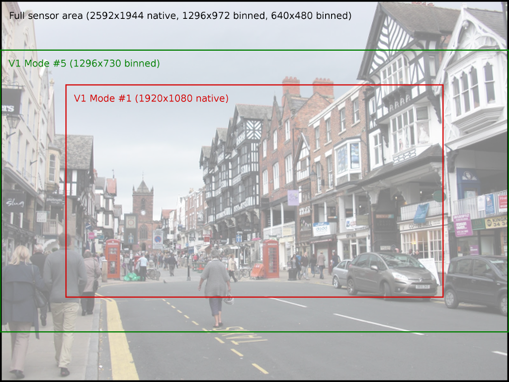
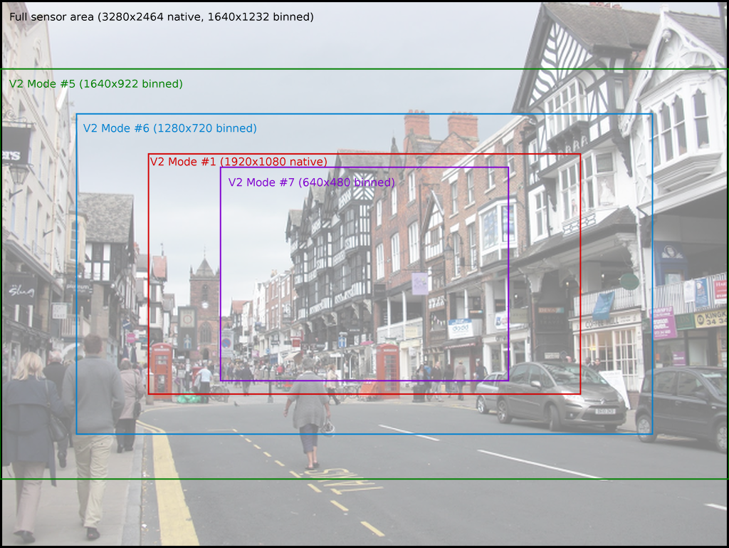
Modes with full field of view (FoV) capture images from the whole area of the camera’s sensor (2592x1944 pixels for the V1 camera, 3280x2464 for the V2 camera). Modes with partial FoV capture images just from the center of the sensor. The combination of FoV limiting, and binning is used to achieve the requested resolution.
The image below illustrates the difference between full and partial field of view for the V1 camera:
While the various fields of view for the V2 camera are illustrated in the following image:
You can manually select the sensor’s mode with the sensor_mode parameter in
the PiCamera constructor, using one of the values from the # column in
the tables above. This parameter defaults to 0, indicating that the mode should
be selected automatically based on the requested resolution
and framerate. The rules governing which sensor mode is
selected are as follows:
- The capture mode must be acceptable. All modes can be used for video
recording, or for image captures from the video port (i.e. when
use_video_port is
Truein calls to the various capture methods). Image captures when use_video_port isFalsemust use an image mode (of which only two exist, both with the maximum resolution). - The closer the requested
resolutionis to the mode’s resolution, the better. Downscaling from a higher sensor resolution to a lower output resolution is preferable to upscaling from a lower sensor resolution to a higher output resolution. - The requested
framerateshould be within the range of the sensor mode. - The closer the aspect ratio of the requested
resolutionto the mode’s resolution, the better. Attempts to set resolutions with aspect ratios other than 4:3 or 16:9 (which are the only ratios directly supported by the modes in the tables above), result in the selection of the mode which maximizes the resulting field of view (FoV).
Here are a few examples for the V1 camera module to clarify the operation of this process:
- If you set the
resolutionto 1024x768 (a 4:3 aspect ratio), and theframerateto anything less than 42fps, the 1296x972 mode (4) will be selected, and the GPU will downscale the result to 1024x768. - If you set the
resolutionto 1280x720 (a 16:9 wide-screen aspect ratio), and theframerateto anything less than 49fps, the 1296x730 mode (5) will be selected and downscaled appropriately. - Setting the
resolutionto 1920x1080 and theframerateto 30fps exceeds the resolution of both the 1296x730 and 1296x972 modes (i.e. they would require upscaling), so the 1920x1080 mode (1) is selected instead, despite it having a reduced FoV. - A
resolutionof 800x600 and aframerateof 60fps will select the 640x480 60fps mode, even though it requires upscaling because the algorithm considers the framerate to take precedence in this case. - Any attempt to capture an image without using the video port will (temporarily) select the 2592x1944 mode while the capture is performed (this is what causes the flicker you sometimes see when a preview is running while a still image is captured).
| Resolution | Framerate (fps) | Result |
|---|---|---|
| 1024x768 (a 4:3 aspect ratio) | < 42 | The 1296x972 mode (4) will be selected, and the GPU will downscale the result to 1024x768. |
| 1280x720 (a 16:9 wide-screen aspect ratio) | < 49 | The 1296x730 mode (5) will be selected and downscaled appropriately. |
| 1920x1080 | 30 | This exceeds the resolution of both the 1296x730 and 1296x972 modes (i.e. they would require upscaling), so the 1920x1080 mode (1) is selected instead, despite it having a reduced FoV. |
| 800x600 | 60 | This selects the 640x480 60fps mode, even though it requires upscaling because the algorithm considers the framerate to take precedence in this case. |
Any attempt to capture an image without using the video port will (temporarily) select the 2592x1944 mode while the capture is performed (this is what causes the flicker you sometimes see when a preview is running while a still image is captured).
6.3. Hardware Limits
The are additional limits imposed by the GPU hardware that performs all image and video processing:
- The maximum resolution for MJPEG recording depends partially on GPU
memory. If you get “Out of resource” errors with MJPEG recording at high
resolutions, try increasing
gpu_memin/boot/config.txt. - The maximum horizontal resolution for default H264 recording is 1920 (this is a limit of the H264 block in the GPU). Any attempt to record H264 video at higher horizontal resolutions will fail.
- The maximum resolution of the V2 camera may require additional GPU memory
when operating at low framerates (<1fps). If you encounter “out of resources” errors when
attempting long-exposure captures with a V2 module, increase
gpu_memin/boot/config.txt. - The maximum resolution of the V2 camera can also cause issues with previews.
Currently, picamera runs previews at the same resolution as captures
(equivalent to
-fpinraspistill). To achieve full resolution operation with the V2 camera module, you may need to increasegpu_memin/boot/config.txt, or configure the preview to use a lowerresolutionthan the camera itself. - The maximum framerate of the camera depends on several factors. With overclocking, 120fps has been achieved on a V2 module, but 90fps is the maximum supported framerate.
- The maximum exposure time is currently 6 seconds on the V1 camera
module, and 10 seconds on the V2 camera module. Remember that exposure
time is limited by framerate, so you need to set an extremely slow
frameratebefore settingshutter_speed.
6.4. MMAL
The MMAL layer below picamera provides a greatly simplified interface to the camera firmware running on the GPU. Conceptually, it presents the camera with three “ports”: the still port, the video port, and the preview port. The following sections describe how these ports are used by picamera and how they influence the camera’s behaviour.
6.4.1. The Still Port
Whenever the still port is used to capture images, it (briefly) forces the camera’s mode to one of the two supported still modes (see Sensor Modes), meaning that images are captured using the full area of the sensor. It also uses a strong noise reduction algorithm on captured images so that they appear higher quality.
The still port is used by the various capture() methods when
their use_video_port parameter is False (which it is by default).
6.4.2. The Video Port
The video port is somewhat simpler in that it never changes the camera’s mode.
The video port is used by the start_recording() method (for
recording video), and also by the various capture()
methods when their use_video_port parameter is True. Images captured from
the video port tend to have a “grainy” appearance, much more akin to a video
frame than the images captured by the still port. This is because the still port
uses a stronger noise reduction algorithm than the video port.
6.4.3. The Preview Port
The preview port operates more or less identically to the video port. The
preview port is always connected to some form of output to ensure that the
auto-gain algorithm can run. When an instance of PiCamera is
constructed, the preview port is initially connected to an instance of
PiNullSink. When start_preview() is called, this null
sink is destroyed and the preview port is connected to an instance of
PiPreviewRenderer. The reverse occurs when
stop_preview() is called.
6.4.4. Pipelines
This section provides some detail about the MMAL pipelines picamera constructs in response to various method calls.
The firmware provides various encoders which can be attached to the still and video ports for the purpose of producing output (e.g. JPEG images or H.264 encoded video). A port can have a single encoder attached to it at any given time (or nothing if the port is not in use).
Encoders are connected directly to the still port. For example, when capturing a picture using the still port, the camera’s state conceptually moves through these states:

As you have probably noticed in the diagram above, the video port is a little more complex. In order to permit simultaneous video recording and image capture via the video port, a “splitter” component is permanently connected to the video port by picamera, and encoders are in turn attached to one of its four output ports (numbered 0, 1, 2, and 3). Hence, when recording video the camera’s setup looks like this:

And when simultaneously capturing images via the video port whilst recording, the camera’s configuration moves through the following states:

When the resize parameter is passed to one of the methods above, a
resizer component is placed between the camera’s ports and the encoder, causing
the output to be resized before it reaches the encoder. This is particularly
useful for video recording, as the H.264 encoder cannot cope with full
resolution input (the GPU hardware can only handle frame widths up to 1920
pixels). So, when performing full frame video recording, the camera’s setup
looks like this:

Finally, when performing unencoded captures an encoder is obviously not required. Instead, data is taken directly from the camera’s ports. However, various firmware limitations require adjustments within the pipeline in order to achieve the requested encodings.
For example, in older firmwares the camera’s still port cannot be configured for RGB output (due to a faulty buffer size check), but they can be configured for YUV output. So in this case, picamera configures the still port for YUV output, attaches a resizer (configured with the same input and output resolution), then configures the resizer’s output for RGBA (the resizer doesn’t support RGB for some reason). It then runs the capture and strips the redundant alpha bytes off the data.
Recent firmwares fix the buffer size check, so with these picamera will simply configure the still port for RGB output (since 1.11):

6.4.5. Encodings
The ports used to connect MMAL components together pass image data around in particular encodings. Often, this is the YUV420 encoding, this is the “preferred” internal format for the pipeline, and on rare occasions it’s RGB (RGB is a large and rather inefficient format). However, there is another format available, called the “OPAQUE” encoding.
“OPAQUE” is the most efficient encoding to use when connecting MMAL components as it simply passes pointers (?) around under the hood rather than full frame data (as such it’s not really an encoding at all, but it’s treated as such by the MMAL framework). However, not all OPAQUE encodings are equivalent:
- The preview port’s OPAQUE encoding contains a single image.
- The video port’s OPAQUE encoding contains two images. These are used for motion estimation by various encoders.
- The still port’s OPAQUE encoding contains strips of a single image.
- The JPEG image encoder accepts the still port’s OPAQUE strips format.
- The MJPEG video encoder does not accept the OPAQUE strips format, only the single and dual image variants provided by the preview or video ports.
- The H264 video encoder in older firmwares only accepts the dual image OPAQUE format (it will accept full-frame YUV input instead though). In newer firmwares it now accepts the single image OPAQUE format too, presumably constructing the second image itself for motion estimation.
- The splitter accepts single or dual image OPAQUE input, but only outputs single image OPAQUE input, or YUV. In later firmwares it also supports RGB or BGR output.
- The VPU resizer (
MMALResizer) theoretically accepts OPAQUE input (though the author hasn’t managed to get this working at the time of writing) but will only produce YUV, RGBA, and BGRA output, not RGB or BGR. - The ISP resizer (
MMALISPResizer, not currently used by picamera’s high level API, but available from themmalobjlayer) accepts OPAQUE input, and will produce almost any unencoded output, including YUV, RGB, BGR, RGBA, and BGRA, but not OPAQUE.
The mmalobj layer, introduced in picamera 1.11, is aware of
these OPAQUE encoding differences and attempts to configure connections between
components using the most efficient formats possible. However, it is not aware
of firmware revisions, so if you’re playing with MMAL components via this layer
be prepared to do some tinkering to get your pipeline working.
Please note that the description above is MMAL’s greatly simplified
presentation of the imaging pipeline. This is far removed from what actually
happens at the GPU’s ISP level (described roughly in earlier sections - link).
However, as MMAL is the API under-pinning the picamera library (along with the
official raspistill and raspivid applications) it is worth
understanding.
In other words, by using picamera you are passing through at least two abstraction layers, which necessarily obscure (but hopefully simplify) the “true” operation of the camera.